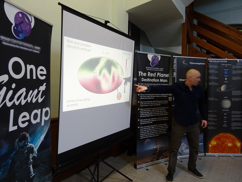
The March 2026 meeting of Keighley astronomical society saw a return visit by Chris Davies, a Professor of Theoretical Geophysics, from the School of Earth and environment at Leeds University. Prof Davies delivered a brand new presentation on the geomagnetic reversals in planet Earth’s core. His presentation had been specifically put together for his visit to us, and included approximately three weeks of computer modelling videos of these changes put together and collated by his team.

Prof Davis started off with a brief description of what a geomagnetic reversal is. It is a change in the Earth’s dipole magnetic field such that the positions of magnetic north and magnetic south are interchanged (not to be confused with geographic north and geographic south). The Earth’s magnetic field has alternated between periods of normal polarity, in which the predominant direction of the field was the same as the present direction, and reverse polarity, in which it was the opposite. These periods are called chrons.

Reversal occurrences appear to be statistically random. There have been at least 183 reversals over the last 83 million years (thus on average once every ~450,000 years). The latest, the Brunhes–Matuyama reversal, occurred 780,000 years ago with widely varying estimates of how quickly it happened. Some sources estimate the most recent four reversals took on average 7,000 years to occur. Clement (2004) suggests that this duration is dependent on latitude, with shorter durations at low latitudes and longer durations at mid and high latitudes. Others estimate the duration of full reversals to vary from between 2,000 and 12,000 years, although some reversals may be as long as 70,000 years.

There have also been episodes in which the field inverted for only a few hundred years (such as the Laschamp excursion). These events are classified as excursions rather than full geomagnetic reversals. Stable polarity chrons often show large, rapid directional excursions, which occur more often than reversals, and could be seen as failed reversals. During such an excursion, the field reverses in the liquid outer core but not in the solid inner core. Diffusion in the outer core is on timescales of 500 years or less while that of the inner core is longer, around 3,000 years.

History

In the early 20th century, geologists such as Bernard Brunhes first noticed that some volcanic rocks were magnetized opposite to the direction of the local Earth’s field. The first systematic evidence for and time-scale estimate of the magnetic reversals were made by Motonori Matuyama in the late 1920s; he observed that rocks with reversed fields were all of early Pleistocene age or older. At the time, the Earth’s polarity was poorly understood, and the possibility of reversal aroused little interest.
Three decades later, when Earth’s magnetic field was better understood, theories were advanced suggesting that the Earth’s field might have reversed in the remote past. Most paleomagnetic research in the late 1950s included an examination of the wandering of the poles and continental drift. Although it was discovered that some rocks would reverse their magnetic field while cooling, it became apparent that most magnetized volcanic rocks preserved traces of the Earth’s magnetic field at the time the rocks had cooled through the Curie temperature. In the absence of reliable methods for obtaining absolute ages for rocks, it was thought that reversals occurred approximately every million years.

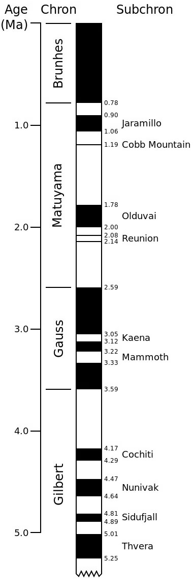
Geomagnetic polarity during the last 5 million years (Pliocene and Quaternary, late Cenozoic Era). Dark areas denote periods where the polarity matches today’s normal polarity; light areas denote periods where that polarity is reversed.

The next major advance in understanding reversals came when techniques for radiometric dating were improved in the 1950s. Allan Cox and Richard Doell, at the United States Geological Survey, wanted to know whether reversals occurred at regular intervals, and they invited geochronologist Brent Dalrymple to join their group. They produced the first magnetic-polarity time scale in 1959. As they accumulated data, they continued to refine this scale in competition with Don Tarling and Ian McDougall at the Australian National University. A group led by Neil Opdyke at the Lamont–Doherty Earth Observatory showed that the same pattern of reversals was recorded in sediments from deep-sea cores.

During the 1950s and 1960s information about variations in the Earth’s magnetic field was gathered largely by means of research vessels, but the complex routes of ocean cruises rendered the association of navigational data with magnetometer readings difficult. Only when data were plotted on a map did it become apparent that remarkably regular and continuous magnetic stripes appeared on the ocean floors.

In 1963, Frederick Vine and Drummond Matthews provided a simple explanation by combining the seafloor spreading theory of Harry Hess with the known time scale of reversals: sea floor rock is magnetized in the direction of the field when it is formed. Thus, sea floor spreading from a central ridge will produce pairs of magnetic stripes parallel to the ridge. Canadian L. W. Morley independently proposed a similar explanation in January 1963, but his work was rejected by the scientific journals Nature and Journal of Geophysical Research, and remained unpublished until 1967, when it appeared in the literary magazine Saturday Review. The Morley–Vine–Matthews hypothesis was the first key scientific test of the seafloor spreading theory of continental drift.

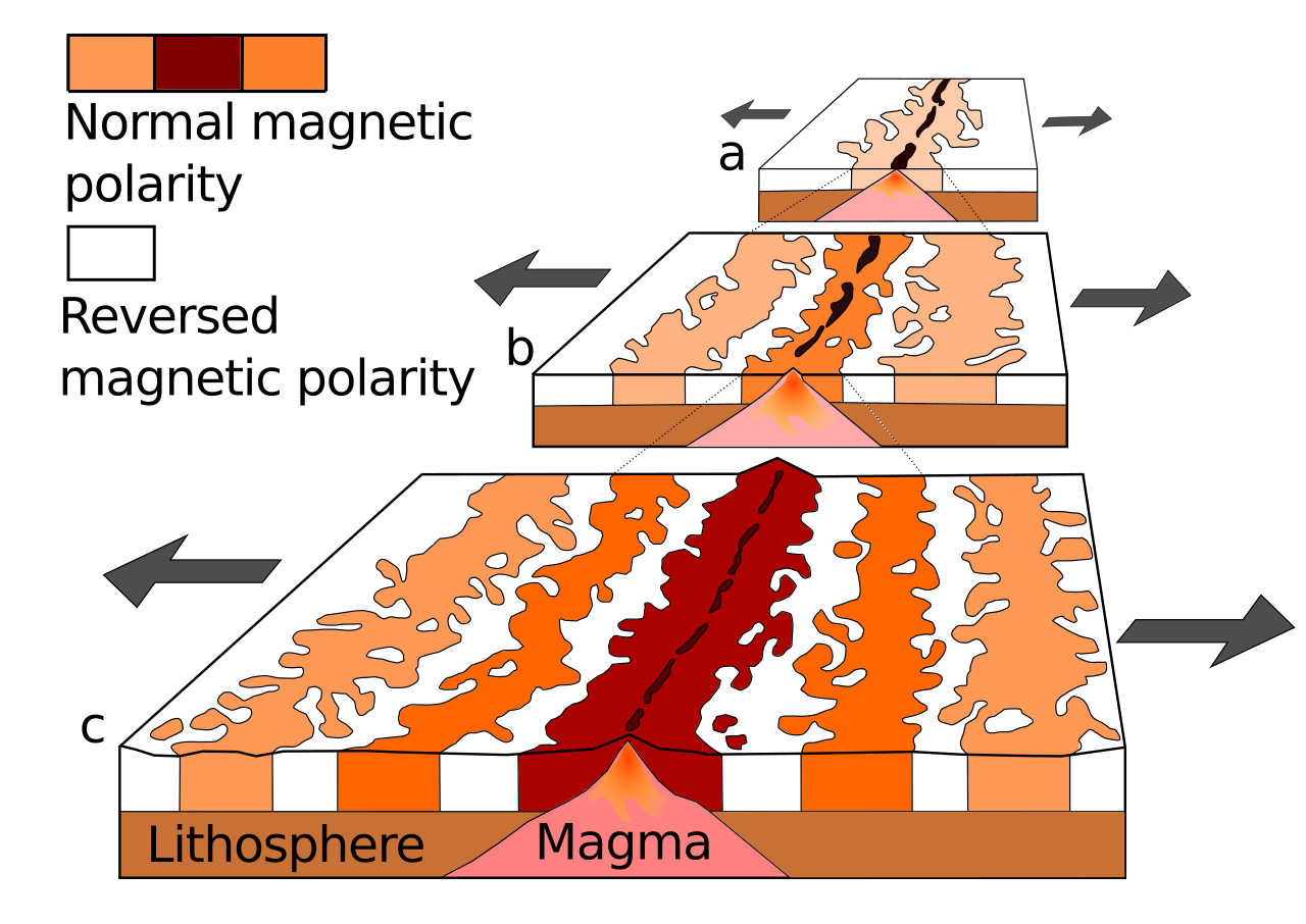
A theoretical model of the formation of magnetic striping. New oceanic crust forming continuously at the crest of the mid-ocean ridge cools and becomes increasingly older as it moves away from the ridge crest with seafloor spreading:

Past field reversals are recorded in the solidified ferrimagnetic minerals of consolidated sedimentary deposits or cooled volcanic flows on land. Beginning in 1966, Lamont–Doherty Geological Observatory scientists found that the magnetic profiles across the Pacific-Antarctic Ridge were symmetrical and matched the pattern in the north Atlantic’s Reykjanes ridge. The same magnetic anomalies were found over most of the world’s oceans, which permitted estimates for when most of the oceanic crust had developed.

Observing past fields

Because no existing unsubducted sea floor (or sea floor thrust onto continental plates) is more than about 180 million years (Ma) old, other methods are necessary for detecting older reversals. Most sedimentary rocks incorporate minute amounts of iron-rich minerals, whose orientation is influenced by the ambient magnetic field at the time at which they formed. These rocks can preserve a record of the field if it is not later erased by chemical, physical or biological change.

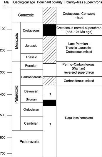
Geomagnetic polarity since the middle Jurassic. Dark areas denote periods where the polarity matches today’s polarity, while light areas denote periods where that polarity is reversed. The Cretaceous Normal superchron is visible as the broad, uninterrupted black band near the middle of the image.

Because Earth’s magnetic field is a global phenomenon, similar patterns of magnetic variations at different sites may be used to help calculate age in different locations. The past four decades of paleomagnetic data about seafloor ages (up to ~250 Ma) has been useful in estimating the age of geologic sections elsewhere. While not an independent dating method, it depends on “absolute” age dating methods like radioisotopic systems to derive numeric ages. It has become especially useful when studying metamorphic and igneous rock formations where index fossils are seldom available.

Geomagnetic polarity time scale

Through analysis of seafloor magnetic anomalies and dating of reversal sequences on land, paleomagnetists have been developing a Geomagnetic Polarity Time Scale. The current time scale contains 184 polarity intervals in the last 83 million years (and therefore 183 reversals).

Changing frequency over time

The rate of reversals in the Earth’s magnetic field has varied widely over time. Around 72 Ma, the field reversed 5 times in a million years. In a 4-million-year period centered on 54 Ma, there were 10 reversals; at around 42 Ma, 17 reversals took place in the span of 3 million years. In a period of 3 million years centering on 24 Ma, 13 reversals occurred. No fewer than 51 reversals occurred in a 12-million-year period, centering on 15 Ma. Two reversals occurred during a span of 50,000 years. These eras of frequent reversals have been counterbalanced by a few “superchrons”: long periods when no reversals took place.

Superchrons

A superchron is a polarity interval lasting at least 10 million years. There are two well-established superchrons, the Cretaceous Normal Superchron and the Kiaman Superchron. A third candidate, the Moyero Superchron, is more controversial. The Jurassic Quiet Zone in ocean magnetic anomalies was once thought to represent a superchron but is now attributed to other causes.

The Cretaceous Normal Superchron (also called the Cretaceous Superchron or C34) lasted for 37 million years, from about 120 to 83 million years ago, including stages of the Cretaceous period from the Aptian through the Santonian. The frequency of magnetic reversals steadily decreased prior to the period, reaching its low point (no reversals) during the period. Between the Cretaceous Normal and the present, the frequency has generally increased slowly.

The Kiaman Reverse Superchron lasted from approximately the late Carboniferous to the late Permian, or for more than 50 million years, from around 312 to 262 million years ago. The magnetic field had reversed polarity. The name “Kiaman” derives from the Australian town of Kiama, where some of the first geological evidence of the superchron was found in 1925.

The Ordovician is suspected to have hosted another superchron, called the Moyero Reverse Superchron, lasting more than 20 million years (485 to 463 million years ago). Thus far, this possible superchron has only been found in the Moyero river section north of the polar circle in Siberia. Moreover, the best data from elsewhere in the world do not show evidence for this superchron. Certain regions of ocean floor, older than 160 Ma, have low-amplitude magnetic anomalies that are hard to interpret.

They are found off the east coast of North America, the northwest coast of Africa, and the western Pacific. They were once thought to represent a superchron called the Jurassic Quiet Zone, but magnetic anomalies are found on land during this period. The geomagnetic field is known to have low intensity between about 130 Ma and 170 Ma, and these sections of ocean floor are especially deep, causing the geomagnetic signal to be attenuated between the seabed and the surface.

Statistical properties

Several studies have analysed the statistical properties of reversals in the hope of learning something about their underlying mechanism. The discriminating power of statistical tests is limited by the small number of polarity intervals. Nevertheless, some general features are well established. In particular, the pattern of reversals is random. There is no correlation between the lengths of polarity intervals. There is no preference for either normal or reversed polarity, and no statistical difference between the distributions of these polarities. This lack of bias is also a robust prediction of dynamo theory.
There is no rate of reversals, as they are statistically random. The randomness of the reversals is inconsistent with periodicity, but several authors have claimed to find periodicity. However, these results are probably artefacts of an analysis using sliding windows to attempt to determine reversal rates.

Most statistical models of reversals have analysed them in terms of a Poisson process or other kinds of renewal process. A Poisson process would have, on average, a constant reversal rate, so it is common to use a non-stationary Poisson process. However, compared to a Poisson process, there is a reduced probability of reversal for tens of thousands of years after a reversal. This could be due to an inhibition in the underlying mechanism, or it could just mean that some shorter polarity intervals have been missed. A random reversal pattern with inhibition can be represented by a gamma process. In 2006, a team of physicists at the University of Calabria found that the reversals also conform to a Lévy distribution, which describes stochastic processes with long-ranging correlations between events in time. The data are also consistent with a deterministic, but chaotic, process.

Duration

Most estimates for the duration of a polarity transition are between 1,000 and 10,000 years, but some estimates are as quick as a human lifetime. During a transition, the magnetic field will not vanish completely, but many poles might form chaotically in different places during reversal, until it stabilizes again.

Studies of 16.7-million-year-old lava flows on Steens Mountain, Oregon, indicate that the Earth’s magnetic field is capable of shifting at a rate of up to 6 degrees per day. This was initially met with scepticism from paleomagnetists. Even if changes occur that quickly in the core, the mantle—which is a semiconductor—is thought to remove variations with periods less than a few months. A variety of possible rock magnetic mechanisms were proposed that would lead to a false signal. That said, paleomagnetic studies of other sections from the same region (the Oregon Plateau flood basalts) give consistent results. It appears that the reversed-to-normal polarity transition that marks the end of Chron C5Cr (16.7 million years ago) contains a series of reversals and excursions.

In addition, geologists Scott Bogue of Occidental College and Jonathan Glen of the US Geological Survey, sampling lava flows in Battle Mountain, Nevada, found evidence for a brief, several-year-long interval during a reversal when the field direction changed by over 50 degrees. The reversal was dated to approximately 15 million years ago. In 2018, researchers reported a reversal lasting only 200 years. A 2019 paper estimates that the most recent reversal, 780,000 years ago, lasted 22,000 years.

Causes

The magnetic field of the Earth, and of other planets that have magnetic fields, is generated by dynamo action in which convection of molten iron in the planetary core generates electric currents, which in turn give rise to magnetic fields. In simulations of planetary dynamos, reversals often emerge spontaneously from the underlying dynamics. For example, Gary Glatzmaier and collaborator Paul Roberts of UCLA ran a numerical model of the coupling between electromagnetism and fluid dynamics in the Earth’s interior. Their simulation reproduced key features of the magnetic field over more than 40,000 years of simulated time, and the computer-generated field reversed itself. Global field reversals at irregular intervals have also been observed in the laboratory liquid metal experiment “VKS2”.

NASA computer simulation using the model of Glatzmaier and Roberts. The tubes represent magnetic field lines, blue when the field points towards the center and yellow when away. The rotation axis of the Earth is centered and vertical. The dense clusters of lines are within the Earth’s core.

In some simulations, this leads to an instability in which the magnetic field spontaneously flips over into the opposite orientation. This scenario is supported by observations of the solar magnetic field, which undergoes spontaneous reversals every 9–12 years. With the Sun it is observed that the solar magnetic intensity greatly increases during a reversal, whereas reversals on Earth seem to occur during periods of low field strength.

Some scientists, such as Richard A. Muller, think that geomagnetic reversals are not spontaneous processes but rather are triggered by external events that directly disrupt the flow in the Earth’s core. Proposals include impact events or internal events such as the arrival of continental slabs carried down into the mantle by the action of plate tectonics at subduction zones or the initiation of new mantle plumes from the core-mantle boundary. Supporters of this hypothesis hold that any of these events could lead to a large scale disruption of the dynamo, effectively turning off the geomagnetic field.

Because the magnetic field is stable in either the present north–south orientation or a reversed orientation, they propose that when the field recovers from such a disruption it spontaneously chooses one state or the other, such that half the recoveries become reversals. This proposed mechanism does not appear to work in a quantitative model, and the evidence from stratigraphy for a correlation between reversals and impact events is weak. There is no evidence for a reversal connected with the impact event that caused the Cretaceous–Paleogene extinction event.

Effects on biosphere

Shortly after the first geomagnetic polarity time scales were produced, scientists began exploring the possibility that reversals could be linked to extinction events. Many such arguments were based on an apparent periodicity in the rate of reversals, but more careful analyses show that the reversal record is not periodic. It may be that the ends of superchrons have caused vigorous convection leading to widespread volcanism, and that the subsequent airborne ash caused extinctions. Tests of correlations between extinctions and reversals are difficult for several reasons. Larger animals are too scarce in the fossil record for good statistics, so paleontologists have analysed microfossil extinctions. Even microfossil data can be unreliable if there are hiatuses in the fossil record. It can appear that the extinction occurs at the end of a polarity interval when the rest of that polarity interval was simply eroded away. Statistical analysis shows no evidence for a correlation between reversals and extinctions.

Most proposals tying reversals to extinction events assume that the Earth’s magnetic field would be much weaker during reversals. Possibly the first such hypothesis was that high-energy particles trapped in the Van Allen radiation belt could be liberated and bombard the Earth. Detailed calculations confirm that if the Earth’s dipole field disappeared entirely (leaving the quadrupole and higher components), most of the atmosphere would become accessible to high-energy particles but would act as a barrier to them, and cosmic ray collisions would produce secondary radiation of beryllium-10 or chlorine-36. A 2012 German study of Greenland ice cores showed a peak of beryllium-10 during a brief complete reversal 41,000 years ago, which led to the magnetic field strength dropping to an estimated 5% of normal during the reversal. There is evidence that this occurs both during secular variation and during reversals.

A hypothesis by McCormac and Evans assumes that the Earth’s field disappears entirely during reversals. They argue that the atmosphere of Mars may have been eroded away by the solar wind because it had no magnetic field to protect it. They predict that ions would be stripped away from Earth’s atmosphere above 100 km. Paleointensity measurements show that the magnetic field has not disappeared during reversals. Based on paleointensity data for the last 800,000 years, the magnetopause is still estimated to have been at about three Earth radii during the Brunhes–Matuyama reversal. Even if the internal magnetic field did disappear, the solar wind can induce a magnetic field in the Earth’s ionosphere sufficient to shield the surface from energetic particles.